Anthropocene Coasts

Volume 5, 2022

Numerical investigation of the wave interaction with flexible vegetation: model setup and validation for a single stem study case

Abstract

Aquatic flexible vegetation plays a very important role in ecosystem, and has been widely used in river or coastal bank revetment. Flexible vegetation contributes to wave attenuation and soil retention. In this study, a fluid-structure bidirectional coupled numerical model (FSC model) was developed based on the codes in-house software HydroFlow^@ to study the interaction between water flow and flexible vegetation. The water wave was simulated using the non-hydrostatic numerical model. Based on the nonlinear theory of elastic thin rod, a dynamic numerical model of flexible vegetation (FV model) was developed using the Finite Element Method (FEM) to simulate the large bending deformation and finite extension of a thin rod. A domain extension method was used to transfer the contact force between waves and the vegetation stem in the coupling process. The FSC model was validated using available experimental results focusing on a single stem dynamic simulation coupling with the free surface open channel flow simulation. The numerical results were in good agreements with the experiments. Relative errors of maximum deflection were less than 10%. Asymmetrical bending during a wave period were captured well compared with the measurements.

Introduction

Compared to conventional “hard” structures, such as seawall and breakwater, ecological vegetation revetment system can not only resist coastal disasters by attenuating wave energy and promote sediment deposition, but also improve coastal resilience. It is more in line with the sustainable development concept of harmonious coexistence between mankind and nature.

The methods to study the wave attenuation ability of ecological vegetation revetment system include the field experiments, the laboratory experiment and the computational model. The first two ways are extremely expensive to perform a series of experiments and require a large number of testing facilities. The computational model has become an important way to investigate the mechanism of wave-vegetation interaction. Vegetation can be classified as rigid vegetation and flexible vegetation according to the stiffness. Compared with the study on the wave attenuation and current resistance by the flexible vegetation, e.g., the seaweed bed, the computational model of rigid vegetation represented by mangrove is relatively mature. There are two main challenges in the development of numerical models of simulating the interaction between waves and flexible vegetation including the bidirectional interaction.

The first challenge is how to simulate the dynamic response process of the large flexible vegetation deflection induced by the water flow. The real flexible vegetation generally has different physical characteristics along the axial direction. Accurately generalizing the physical characteristics using parameters as few as possible is quite important and practical. The Cauchy number (Ca) and the buoyancy number (B) were used as the main criteria for extended and bent flexible vegetation according to different computational models (Nikora 2010; Luhar and Nepf 2011; Marjoribanks et al. 2014). The N-Pendula model were formulated in rules of the local force balance for each segment without considering the elastics of vegetation itself (Abdelrhman 2007; Zeller et al. 2014; Tahvildari 2016). In a different spirit, one model was proposed to establish and solve the large deflection plane deformation equation along the arc coordinate along the vegetation length based on the Euler-Bernoulli elastic beam theory by introducing a higher order curvature description (Dijkstra and Uittenbogaard 2010; Li and Xie 2011; Kubrak et al. 2012). Due to the real complex flow conditions and vegetation characteristics, spatial large deflection deformation and finite extension deformation should be considered. The spatial elastic thin rod theory is more suitable for the bending, shear, torsion and even knotting of the elastic thin rod and other complex spatial geometric nonlinear deformation. Meanwhile, it is easy to deal with the extensible deformation, and can be used to model the real aquatic flexible vegetation. Garrett (1982), Ran (2000) and Zhang et al. (2019) proposed and improved the statics and dynamics finite element numerical models applicable to the large deflection deformation of extensible elastic thin rod in the global coordinate system. Mattis et al. (2019) and Chen and Zou (2019) applied this kind of model to investigate the dynamic response of flexible vegetation forced by water waves.

Another challenge of the numerical simulation is that the kinematics of the flexible vegetation will induce more complex water flows compared to those induced by the rigid vegetation. Luhar and Nepf (2011, 2016) studied the response process of flexible analog blades under the open channel flows and wave-induced oscillatory flows, respectively. They calculated the forces through the measured flow velocities along the blades, but did not consider the effect of flexible blades reacting on the water flow. It is necessary to develop a suitable and efficient fluid-solid bidirectional coupling computational model to study this coupling process. In the coupling process, it is very costly and unnecessary to simulate the entire boundary layer flow around each plant stem. Therefore, the Immersion Boundary Method (IBM) or the immersed structure approach are generally adopted along the centerline of flexible vegetation. This kind of coupled model takes the center line of the flexible rod as the virtual boundary, and uses the δ function to interpolate the hydrodynamic force on the stem and redistribute the force into the CFD cells. Chen and Zou (2019) presented a novel coupled flow-vegetation interaction model to resolve the flow and the simultaneous response of the flexible vegetation. The simulation results of the asymmetric displacement of the vegetation motion, the wave height attenuation, and the wave motion within and outside the vegetation patch were in good agreements with measurements. Mattis et al. (2019) presented a computational model to investigate the wave attenuation over flexible vegetation using the immersed-structure method (Mattis et al. 2015). They performed a series of computational experiments to analyze and compare the wave attenuation by means of the wave heights, spectra, and energy with experimental results.

The objective of this paper is to develop and validate a bidirectional coupled fluid-vegetation dynamic model. Compared with previous studies on the numerical simulation of the vegetation flow, the model in this paper has two distinct improvements. Firstly, when modelling the large deflection deformation of the vegetation stem, the inconsistency of vegetation parameters along the axial direction was taken into account in order to promote the consistency of the model to the real vegetation. Secondly, for the semi-analytical method adopted in the domain expansion during the coupling process, the influence of the solid volume fraction on water flow was included in the coupled simulation by implementing the porous media water flow model.

The remainder of this paper is organized as follows. In Section 2, the FSC model is described and implemented. A series of numerical simulations of the open channel flows passing a single stem are carried out. The mesh convergence is verified through comparing the simulated results of three sets of grids with the experiments. In Section 3, the numerical model is applied to simulate the interaction between waves and a single stem. The simulation results are validated by means of experiments. Meanwhile, some discussion on the results is provided in the section. Finally, Section 4 presents conclusions and further proposals.

Model development

Computational Fluid Dynamic (CFD) Model

In the Reynolds-averaged Navier-Stokes equations (RANS) model, the waves are generated by introducing the mass source terms in the governing equation. The basic governing equations of water flow include the continuity equation and the momentum conservation equations. The influence of the flexible vegetation stems on the water flow is modelled by introducing the resistance source terms into the momentum equations based on the porous media numerical model. The codes in-house CFD software HydroFlow® adopts a vertical coordinate transformation to fix the free surface and uneven bottom, i.e., the σ coordinate transformation. The governing equations are formulated as follows,

\partial λ ζ \partial t + \partial λ q x \partial x + \partial λ q y \partial y + \partial λ q σ \partial σ = 0

(1)

\partial λ q x \partial t + \partial λ q x u \partial x + \partial λ q x v \partial y + \partial λ q x w ~ \partial σ = \partial \partial x (ν t H \partial λ q x \partial x) + \partial \partial y (ν t H \partial λ q x \partial y) + 1 D \partial \partial σ (ν t V D \partial λ q x \partial σ) - g D \partial λ ζ \partial x - D ρ \partial λ p n \partial x - F s u m h d x D ρ

(2)

\partial λ q y \partial t + \partial λ q y u \partial x + \partial λ q y v \partial y + \partial λ q y w ~ \partial σ = \partial \partial x (ν t H \partial λ q y \partial x) + \partial \partial y (ν t H \partial λ q y \partial y) + 1 D \partial \partial σ (ν t V D \partial λ q y \partial σ) - g D \partial λ ζ \partial y - D ρ \partial λ p n \partial y - F s u m h d y D ρ

(3)

\partial λ q z \partial t + \partial λ q z u \partial x + \partial λ q z v \partial y + \partial λ q z w ~ \partial σ = \partial \partial x (ν t H \partial λ q z \partial x) + \partial \partial y (ν t H \partial λ q z \partial y) + 1 D \partial \partial σ (ν t V D \partial λ q z \partial σ) - 1 ρ \partial λ p n \partial σ - F s u m h d z D ρ

(4)

where ζ is the water level, λ = 1 − ϕ is the porosity ranging from 0 to 1, ϕ is the solid volume fraction of the flexible vegetation and p_n is the dynamic pressure. $F_{h d}^{s u m} = \sum_{n = 1}^{N} F_{h d} = {[\sum_{n = 1}^{N} F_{h d x}, \sum_{n = 1}^{N} F_{h d y}, \sum_{n = 1}^{N} F_{h d z}]}^{T}$ is the reacting force of the flexible vegetation patch on fluid, in which N is the statistical density of vegetation, i.e. the number of stems per area with the unit stems/m²; ρ is the density of fluid; q_x = Du, q_y = Dv, q_z = Dw and $q_{σ} = D \tilde{w}$ are the defined flow variables, in which D is the still water depth, u, v and w are the velocity components corresponding to x, y and z direction; $\tilde{w}$ is the vertical velocity in the σ coordinate.

In the traditional SST k–ω turbulence model proposed by Menter (1994), a term formulating the turbulent kinetic energy generated by the motion of the flexible vegetations is introduced, as follows,

D k D t = τ i j ρ \partial u i \partial x j - β * ω k + \partial \partial x j [(ν + σ k ν t) \partial k \partial x j] + S k, i, j = 1, 2, 3

(5)

D ω D t = γ ρ ν t τ i j \partial u i \partial x j + \partial \partial x j [(ν + σ ω ν t) \partial ω \partial x j] - β ω 2 + S ω + 2 (1 - F 1) σ ω 2 1 ω \partial k \partial x j \partial ω \partial x j, i, j = 1, 2, 3

(6)

where $S_{k} = \frac{1}{2} C_{k p} C_{D} a \sqrt{u_{j} u_{j}} k$ and $S_{ω} = \frac{1}{2} C_{k p} C_{ω p} C_{D} a \sqrt{u_{j} u_{j}} ω$ are the turbulence production and dissipation source terms due to the presence of vegetation; a = b_vN is the vegetation density measured as frontal area per unit volume with a unit of m^− 1 and the parameters C_kp = 1, C_ωp = 3.5 referred to Cheng et al. (2019); The other values of coefficients and the meaning of variables are referred to Menter (1994).

FV model solved using FEM

Based on the spatial elastic thin rod theory, without considering the torsion between cross sections, the governing equations of elastic thin rod motion and finite tension are as follows,

F' + q = ρ r ¨

(7)

M' + r ' | r ' | \times F + m = 0

(8)

r' \cdot r' = 1 + ε

(9)

where $F^{'} = \frac{d F}{d s}$ and $M^{'} = \frac{d M}{d s}$ are respectively the derivative of the resultant force and resultant moment per unit length along the center line with respect to the arc coordinates (s). The force q and moment m per unit length are applied. The superscript notation prime represents the derivative with respect to the arc length, dot represents the derivative with respect to time, and ε is the finite micro extension.

Assuming the flexible vegetation rod is completely immersed in water, the external loads per unit length include the gravity, the hydrostatic force F_s and the hydrodynamic force F_d,

q = w + F s + F d

(10)

The hydrodynamic force F_d consists of the inertial force and the drag force,

F d = q I f + q D f

(11)

where the inertial force $q_{f}^{I} = ρ A_{v} (C_{M} {\dot{V}}_{f}^{N} - C_{m} {\ddot{r}}^{N})$ and the drag force $q_{f}^{D} = \frac{ρ}{2} d_{e} C_{D} (V_{f}^{N} - {\dot{r}}^{N}) | (V_{f}^{N} - {\dot{r}}^{N}) |$ are calculated using the Morrison formula;

A_v is the cross area of the stem, and d_e is the effective diameter of the stem; The parameter A_v and d_e are not constant along the axis line. The superscript N denotes the normal direction of the rod surface; The vector $V_{f}^{N}$ is flow velocity vector including u, v and w components.

FEM is adopted to discretize the governing equations. Galerkin method is used to integrate the discrete differential equations of motion and the extensible control equations within the element cells. The detailed solve process are referred to Ran (2000), Ma (2014), and Zhang et al. (2019).

The domain expansion method

To improve the applicability and accuracy of the coupled numerical model, a domain expansion method using a Gaussian kernel function is adopted to couple the simulations of the water flow and the flexible vegetation dynamics. In the semi-analytic model, the influential domain of the stem on the flow is extended from the local grid containing the discrete vegetation node to a neighbor spherical domain with a diameter D_e = κd_e. The d_e is the characteristic diameter of the vegetation stem, κ is a scalar factor determining the range of the neighboring CFD cells (Wang et al. 2019), and often specified a value in the range of 1–3. The method of kernel function approximation is often used to estimate the field values of random distribution points. The normalized weights (ψ_i, j) can be calculated by the Gaussian kernel $f (R_{i j}, σ) = e^{- {R_{i j}}_{2} / 2 σ^{2}}$ ,

ψ i, j = ⎧⎩⎨⎪⎪⎪⎪ f ( R i j , σ ) Δ V j \sum j = 1 N C f ( R i j , σ ) Δ V j, R i j \leq D e 0, R i j > D e

(12)

where R_ij = ‖X_i − X_j‖ is the distance between the node and the fluid grid, X_i is the position of the ith vegetation node, and X_j is the center coordinates of the jth fluid cell within the expanded sphere domain. The σ = κ₁d_e is the bandwidth of the kernel function, and κ₁ is often specified a value in the range of 1–3 for general kernel approximations. The ΔV_j is the volume of the jth CFD cell, and NC is the number of the neighboring CFD cells.

Once the normalized weights are calculated, the variables needed to be interpolated from CFD cells can be calculated by the formula $ϕ_{f, i} = \sum_{j = 1}^{N C} ψ_{i, j} ϕ_{f, j}$ . Similarly, the variables needed to be fed back to the CFD cells can also be calculated by the formula $ϕ_{f, j} = \sum_{i = 1}^{N O D E S} ψ_{i, j} ϕ_{f, i}$ . The detailed expressions are referred to Wang et al. (2019).

Mesh convergence verification

Based on the physical experiments from Luhar and Nepf (2011), the numerical open channel flume was set up and is shown as Fig. 1. The length (L), width (B) and water depth (h) of the numerical flume were set as 4.0 m, 0.2 m and 0.3 m, respectively. Two flow conditions with uniform velocity U of 0.16 m/s and 0.32 m/s were generated by specifying the inflow discharge. A constant water level was specified at the outlet. Slip boundary condition was set on the side wall. The thin rods of the model vegetation were high density polyethylene (HDPE) plate and silicone foam board (SF). The thickness (t), width (b) and height (l) of both materials were 0.0004 m (SF = 0.0019 m), 0.01 m and 0.25 m, respectively. Accordingly, the elastic modulus (E) was 0.93 GPa and 500 KPa, and the density ρ_v is 975 kg/m³ and 695 kg/m³. The stem was placed at the position x = 1.25 m. The resistance coefficient (C_D) was set a constant value of 1.95.

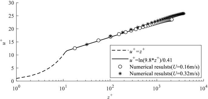
Three sets of grids covering the portion of the vegetation were designed to analyze the convergence of the grids. The size ratio (Δ/d) of grid scale to the stem diameter in the semi-analytical model using the domain extension method varies between 0.1 and 3. In this paper, the size ratio (Δx/b and Δx/b) was 2.5, 1 and 0.5, which was corresponding to the horizontal grid resolution 0.025 m × 0.025 m, 0.01 m × 0.01 m and 0.005 m × 0.005 m. The finite volume method adopted in this paper disperses physical quantities to the center of the CFD cells, so the height of the first-layer grid (Δz) is 0.0025 m. The bottom wall friction velocities u^∗ were respectively 0.007 m/s and 0.013 m/s for the incident flows with free stream velocity 0.16 m/s and 0.32 m/s. The dimensionless height of the nearest grid to the bottom (z⁺ = zu_∗/υ) was 17.68 and 31.95, respectively, which met the limitation of 11.63 for the usability of the wall function. The distribution of the dimensionless streamwise velocity (u⁺ = u/u_∗) in the vertical direction were shown in Fig. 2. It reveals that the vertical distribution of the dimensionless flow velocities u⁺ coincides well with the classic log-law velocity profile.

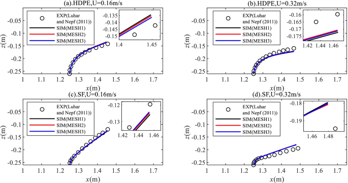
The results of the balance positions are shown in Fig. 3. There are little differences of the simulated deflections using the three sets of grids, which indicates a convergence of the grid resolution. All of the simulated results are in good agreement with the experimental results. According to statistical analysis, the maximum relative error between the simulated free end deflection of three sets of grids and experimental deflection in the z direction of the HDPE stem was about 5.46% in the case with the incident flow velocity 0.16 m/s and 7.97% in the case with the incident flow velocity 0.32 m/s, respectively. For SF stem, the maximum relative errors were 5.13% and 7.70%. Generally, the maximum relative errors of both plates under the two specified flow conditions were below 10%. In the following test cases, MESH2 was used for coupling numerical simulation taking into account both the simulation accuracy and the computational cost.

Model application

The FSC model was used to investigate the interaction of water waves and a single-stem vegetation mimicked by a flexible plate. Meanwhile, the FSC model was further validated by means of comparing with experiments.

Numerical wave generation and validation

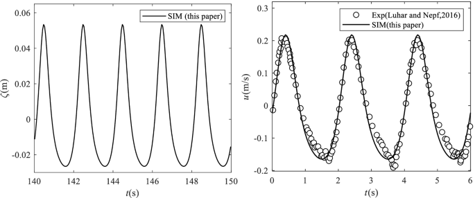
For the physical experiments from Luhar and Nepf (2016), the numerical wave flume was 34.0 m long, 0.2 m wide and 0.3 m deep under the still water level. The experimental sinusoidal wave with the wave height (H_w) 0.08 m, the wave period (T) 2.0 s and the wavelength (λ) 3.256 m was specified in the numerical simulations. The flexible vegetation stem was placed at x/λ ≈ 7 away from the wave generation position. The root segment of the stem was 0.26 m under the free water level. The flow monitoring point was set at 0.15 m upstream of the stem. The geometry of the thin HDPE flat-plate was with a width of 0.02 m and a height of 0.2 m. In the range of x/λ ≈ 5 − 7.5, the grid resolution Δx × Δy = 0.02 m × 0.02 m was used by analyzing the mentioned grid convergence above. The mass source wave generation method was used to generate waves, and the sponge zone was set at the two ends of the numerical flume with a length ranged in 1.5 λ – 2.0 λ to dampen the incident waves (Fig. 4). The sinusoidal wave with the period T = 2.0 s, the wave height H_w = 0.08 m was numerically generated and compared with the measurements. Figure 5 reveals that the simulated velocity waveform is generally consistent with the experimental results but with slight discrepancy during the wave trough phase. The magnitude of the velocity indirectly reflects the force magnitude.

Model results and discussion

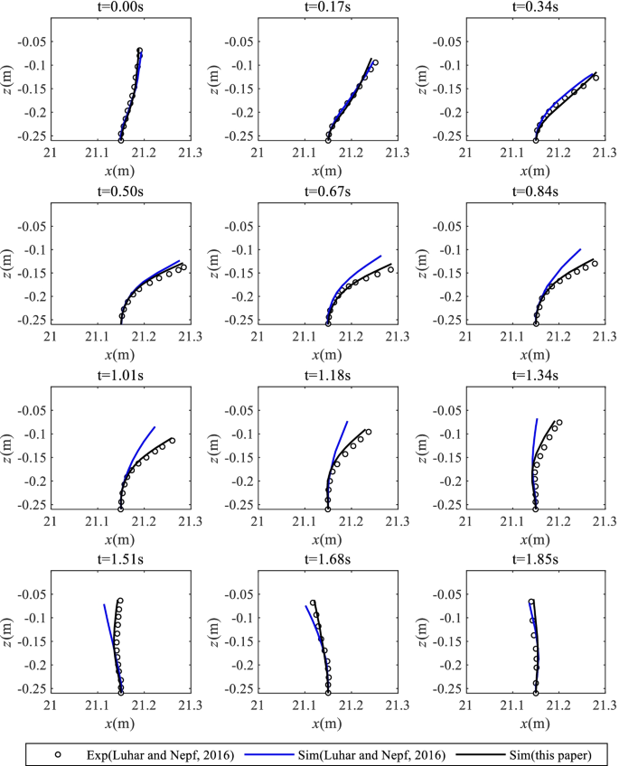
The simulated bending process within a wave period was compared with the experiment, which is shown in Figs. 6 and 7.

Figure 6 reveals the asymmetric trajectory of the free end of the stem during a wave period. The stem leans in the downstream direction due to the asymmetry of the velocity waveform in the flow field. The predicted stem tip excursion in the x direction was 0.169 m which was underestimated 3.4% compared to the experimental result (0.175 m). Maximum deflections in the x direction and z direction in the second half wave period were overestimated 0.002 m and underestimated 0.004 m resulting in the relative errors of 0.01% and − 6.42%. Similarly, Maximum deflections in the x direction and the z direction in the first half wave period were underestimated 0.007 m and 0.0144 m resulting in the relative errors of 0.03% and 9.89%, respectively. In other words, underestimation of the horizontal deflections occurred mainly in the first half wave period. Since the upper part of the stem is in passive motion, the force is mainly concentrated on the lower part of vegetation (Luhar and Nepf 2016). In this paper, Morrison formula (Eq. (11)) is used to calculate the force on vegetation. The main factors determing the force on the vegetation stem are the values of the empirical constant C_D and C_m, and the relative velocity $(V_{f}^{N} - {\dot{r}}^{N})$ . The constant C_D (3.66) and C_m (1.0) were employed in the study cases. Definitely, the drag force is reduced due to the pressure recovery near the free end of stem, therefore the effective C_D and C_m in the simulation is estimated a bit smaller, which led to the underestimation of the stem excursion in the first half wave period. The maximum relative error of deflection in two directions was less than 10%, which is considered to be acceptable.

As shown in Fig. 7, the simulation well captures the stem bending process compared with the experimental results with a higher accuracy than the prediction from Luhar and Nepf (2016). One reason may be that the FSC model adopted in this paper implements a two-way interaction between fluid flows and the vegetation stems by means of feeding the hydrodynamic force back into the fluid body. The model used by Luhar and Nepf (2016) only included a one-way interaction, i.e., the influence of the vegetation stem on the fluid flow being neglected.

Conclusions

In this paper, a 3D FSC model was developed, including flexible vegetation dynamic model, porous media model and domain expansion coupling model. The mesh convergence was verified and the accuracy of this model was preliminary validated in the test case of simulating open channel flow around a single stem. The size ratio of grid size to the stem diameter equals to unit can ensure the model accuracy and the simulation efficiency. This model was furtherly used to investigate the interaction between waves and a single plate. The simulation using the FSC model well predicted asymmetric deflection of the plate forced by regular waves. Compared with experimental results, the relative errors of the simulated maximum deflection of the free end are less than 10%.

In terms of numerical methods, the diameters (D_e) of the sphere domain around the flexible vegetation and the bandwidth (σ) are empirical and lack of quantitative validations. Meanwhile, there are many specific physical application problems needed to be studied and discussed, such as evaluating how the stiffness influence the period of the vegetation vibration under waves, investigating the effects of density, height, rigidity parameters of vegetation patch on the flow velocity and turbulence, and so on. Further research will focus on improving the numerical technique and promoting applications in vegetation flow research in a large spatial scale, e.g., a natural vegetation patch.

Availability of data and materials

The first author, Ms. Caiping Jin ([email protected]) can be contacted for access to the data.

Get Involved

Find out how to contribute to Future Earth Coasts. Join our mailing list for recent updates of the community.